Testing the LABS modules

In the previous post in this series I introduced the LABS problem, and explained some of the relevant properties of the binary sequences. I also sketched out my proposed solution and started work on implementing this solution in SystemVerilog.

In this post I will cover some design verification for the modules we have designed thus far, so that we can be confident of our basic building blocks when we start wiring them together.

You can view the other posts in this series here:

1. Searching for Low Autocorrelation Binary Sequences
2. Testing the LABS modules [This Post]

Design Verification

Verifying RTL designs is a critical part of the design process. Debugging on FPGAs is a tough challenge, so it is important to have other methods of catching bugs and building up confidence in the code. In this blog post we will first develop a high level model of our problem (in this case using Python code); personally I find these models really useful for a few reasons, which I will explain in more detail in the next section. After creating the high-level model we will create a basic handwritten testbench; I normally use these testbenches for two reasons: to verify the basic functionality of the RTL block under test, and to generate waveforms for inspection. The focus of the next blog post will be on writing automated test benches to significantly increase the coverage of our testing.

Python Models

As I mentioned before, I like to write models of the RTL code in a high-level language like Python. Such models can be used to calculate the expected outputs for a given input, which is useful when running simulations later. In a high level model, I can use higher level concepts and libraries, which makes it easier to prove. For example, when working on a DSP signal processing chain I can use built-in maths functions and floating point numbers; or, if I am working on an implementation of a hashfunction I can use the built-in libraries in Python. And finally, we can use the model to verify the output signals in automated testbenches, which can cover a much wider range of inputs than handwritten testbenches.

The listing below shows the Python models for the three RTL modules we developed in the last post: calc_ck, square_accumulate and calc_e. The Python function calc_ck_impl represents the calc_ck module, and the calc_ck function is a convenience function which calculates the second input sequence based on the original sequence.

One downside of using Python is that integer types do not have a fixed width, so we have to use some bit-fiddling using masks to accurately represent the effect of signals with fixed widths in hardware.

 1
 2
 3
 4
 5
 6
 7
 8
 9
10
11
12
13
14
15
16
17
18
19
20
21
22
23
24
25
26
27
28
29
30
31
32
33
34
35
36
37
38
39
40

def __signed_mask(N, val):
    mask = 2**(N-1) - 1
    f = (lambda x: x) if val > 0 else (lambda x: -x) 

    return f(f(val) & mask)

def __unsigned_mask(N, val):
    mask = 2**N - 1
    return val & mask

def square_accumulate(W, a, b):
    a_byte = __signed_mask(8, a)
    b_mask = __unsigned_mask(W, b)
    
    result = a_byte * a_byte + b
    return __unsigned_mask(W, result)

def calc_ck(N, seq, k):
    seq_a = seq
    seq_b = seq >> k

    return calc_ck_impl(N - k, seq_a, seq_b)
    
def calc_ck_impl(W, seq_a, seq_b):
    xnor = ~(seq_a ^ seq_b)
    masked = __unsigned_mask(W, xnor)
    count = int.bit_count(masked)

    pos = count
    neg = W - count

    return pos - neg

def calc_e(N, seq, W = 16):
    ck = [calc_ck(N, seq, ii) for ii in range(1, N)]
    e = 0
    for t in ck:
        e = square_accumulate(W, t, e)

    return e

We can also use pytest to write some unit test for our model, to verify the model. In this case the inputs for the tests are values I worked out by hand to populate the example diagrams in the previous blog post.

 1
 2
 3
 4
 5
 6
 7
 8
 9
10
11
12
13
14
15
16
17
18
19
20
21
22
23
24
25
26
27
28
29
30
31
32
33
34
35
36
37
38
39
40
41
42
43

def test_square_accumulate():
    # Test 0 * 0 + 10 == 10
    assert labs.model.square_accumulate(8, 0, 10) == 10
    # Test 10 * 10 + 0 == 100
    assert labs.model.square_accumulate(8, 10, 0) == 100
    # Test 10 * 10 + 10 = 110
    assert labs.model.square_accumulate(8, 10, 10) == 110
    # Test wider signals
    assert labs.model.square_accumulate(16, 30, 100) == 1000
    # Test overflow
    assert labs.model.square_accumulate(8, 30, 100) == 232
    # Test negative input
    assert labs.model.square_accumulate(8, -8, 0) == 64

def test_calc_ck_impl():
    # Test c_1, c_2, c_3 for the input sequence {-1, 1, 1, -1} => {0, 1, 1, 0}
    # The expected values are c_1 = -1, c_2 = -2, c_3 = 1
    assert labs.model.calc_ck_impl(3, 0b110, 0b011) == -1
    assert labs.model.calc_ck_impl(2, 0b10, 0b01) == -2
    assert labs.model.calc_ck_impl(1, 0b0, 0b0) ==  1

    # Test on 8-bit sequences with some simple rules of thumb:
    # - When all bits equal we expect the result to equal the number of bits.
    # - When all bits are different we expect the result to be equal to minus the number of bits.
    # - When half the bits are the same and half are different we expect the result to be zero.
    assert labs.model.calc_ck_impl(8, 0x00, 0x00) == 8
    assert labs.model.calc_ck_impl(8, 0x0F, 0x00) == 0
    assert labs.model.calc_ck_impl(8, 0x0F, 0xFF) == 0
    assert labs.model.calc_ck_impl(8, 0x00, 0xFF) == -8

def test_calc_ck():
    # Test c_1, c_2, c_3 for the input sequence {-1, 1, 1, -1} => {0, 1, 1, 0}
    # The expected values are c_1 = -1, c_2 = -2, c_3 = 1
    assert labs.model.calc_ck(4, 0b0110, 1) == -1
    assert labs.model.calc_ck(4, 0b0110, 2) == -2
    assert labs.model.calc_ck(4, 0b0110, 3) ==  1

def test_calc_e():
    # Test all sequences of length 4
    expected = [14, 2, 2, 6, 2, 14, 6, 2, 2, 6, 14, 2, 6, 2, 2, 14]
    for ii in range(16):
        assert labs.model.calc_e(4, ii) == expected[ii]
    

Now we have a good model in Python for the RTL modules we are about to test, and we have written some basic unit tests to validate their behaviour. The next step is to hand-write test benches for each of these modules.

Testbenches

The following testbenches are written by hand, using the same test inputs we used above in the unit tests for the Python models. The value of these testbenches is that we can write them quickly and use them to verify the basic functionality of our RTL code, while also generating waveform files which we can inspect.

In this post we will use a tool called Icarus Verilog (also known as iverilog) to run our simulations / testbenches. iverilog is an open source tool which aims to be able to compile all of the Verilog HDL standard, though as of this time the support for recent additions to the specification is limited. With iverilog we can compile our Verilog code into an executable which we can run on our system. We will also use GTKWave to visualise the waveform files which can be generated using iverilog.

Correlation Calculation

The first testbench, for the calc_ck block, is listed below. The testbench creates an instance of calc_ck with a seuence width of 8 bits. It is then tested using four inputs: (0, 0), (15, 0), (15, 255), (0, 255). These are the same inputs we used in the unit test for the Python model, so we know the expected outputs. We are using the $display command to print the output signal z on the commandline, and we are using assert to test that the output matches the results we expect.

 1
 2
 3
 4
 5
 6
 7
 8
 9
10
11
12
13
14
15
16
17
18
19
20
21
22
23
24
25
26
27
28
29
30
31
32
33
34
35
36

module tb_calc_ck;
    localparam period = 10;
    localparam hperiod = period/2;

    reg clk;
    reg [7:0] a, b;
    wire signed [7:0] z;

    calc_ck #(.SEQ_WIDTH(8)) UUT (.clk(clk), .a(a), .b(b), .z(z));

    always #hperiod clk = ~clk;

    initial begin
        $dumpfile("tb_calc_ck.vcd");
        $dumpvars(0,tb_calc_ck);

        clk = 0;
        a = 0; b = 0;
        #period; $display(z);
        assert(z == 8);

        a = 15;
        #period; $display(z);
        assert(z == 0);

        b = 255;
        #period; $display(z);
        assert(z == 0);

        a = 0;
        #period; $display(z);
        assert(z == -8);

        $finish();
    end
endmodule

The testbench can be compiled into an executable using iverilog as follows, and then it can be executed.

1
2
3
4
5
6
7

$ iverilog -g2009 -o tb_calc_ck tb_calc_ck.sv ../rtl/calc_ck.sv
$ ./tb_calc_ck
VCD info: dumpfile tb_calc_ck.vcd opened for output.
   8
   0
   0
  -8

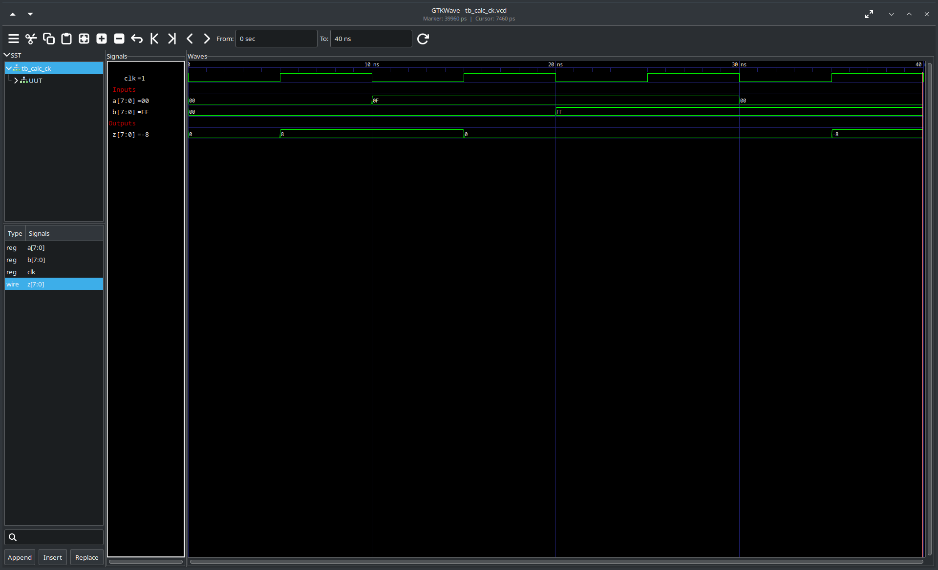
The output from the $display command matches the expected values based on our Python model. We can also use gtkwave to inspect the dumpfile tb_calc_ck.vcd, which contains the waveforms generated by the testbench. The figure below shows these waveforms (you can click on the image to expand it) in GTKWave. In this case the waveform does not show us much that we did not already know, but it can be very useful for more complicated designs. When working with buses it allows you to view all the signals invovled in a bus transactions in a convenient way, when working on FPGA designs for mixed signal applications, the waveform viewers can plot the digital signal as analog trace and when debugging why a simulation is not giving the expected result, it allows you to view signals buried deep inside the hierachy of the design.

Square Accumulate

The second hand-written testbench is for the square_accumulate module. Again we use a series of inputs which we have already verified using the Python model, and we use $display and assert to print and check the output from the unit-under-test.

 1
 2
 3
 4
 5
 6
 7
 8
 9
10
11
12
13
14
15
16
17
18
19
20
21
22
23
24
25
26
27
28
29
30
31
32
33
34
35
36
37
38
39
40
41
42
43
44
45
46

module tb_square_accumulate;
    localparam period = 10;
    localparam hperiod = period/2;

    reg clk;
    reg signed [7:0] a;
    reg [15:0] b;
    wire [15:0] z;

    square_accumulate UUT (.clk(clk), .a(a), .b(b), .z(z));

    always #hperiod clk = ~clk;

    initial begin
        $dumpfile("tb_square_accumulate.vcd");
        $dumpvars(0,tb_square_accumulate);

        clk = 0;
        
        a = 0; b = 0;
        #period; $display(z);
        assert(z == 0);

        b = 10;
        #period; $display(z);
        assert(z == 10);

        a = 10; b = 0;
        #period; $display(z);
        assert(z == 100);

        b = 10;
        #period; $display(z);
        assert(z == 110);

        a = 30; b = 100;
        #period; $display(z);
        assert(z == 1000);

        a = -8; b = 0;
        #period; $display(z);
        assert(z == 64);

        $finish();
    end
endmodule

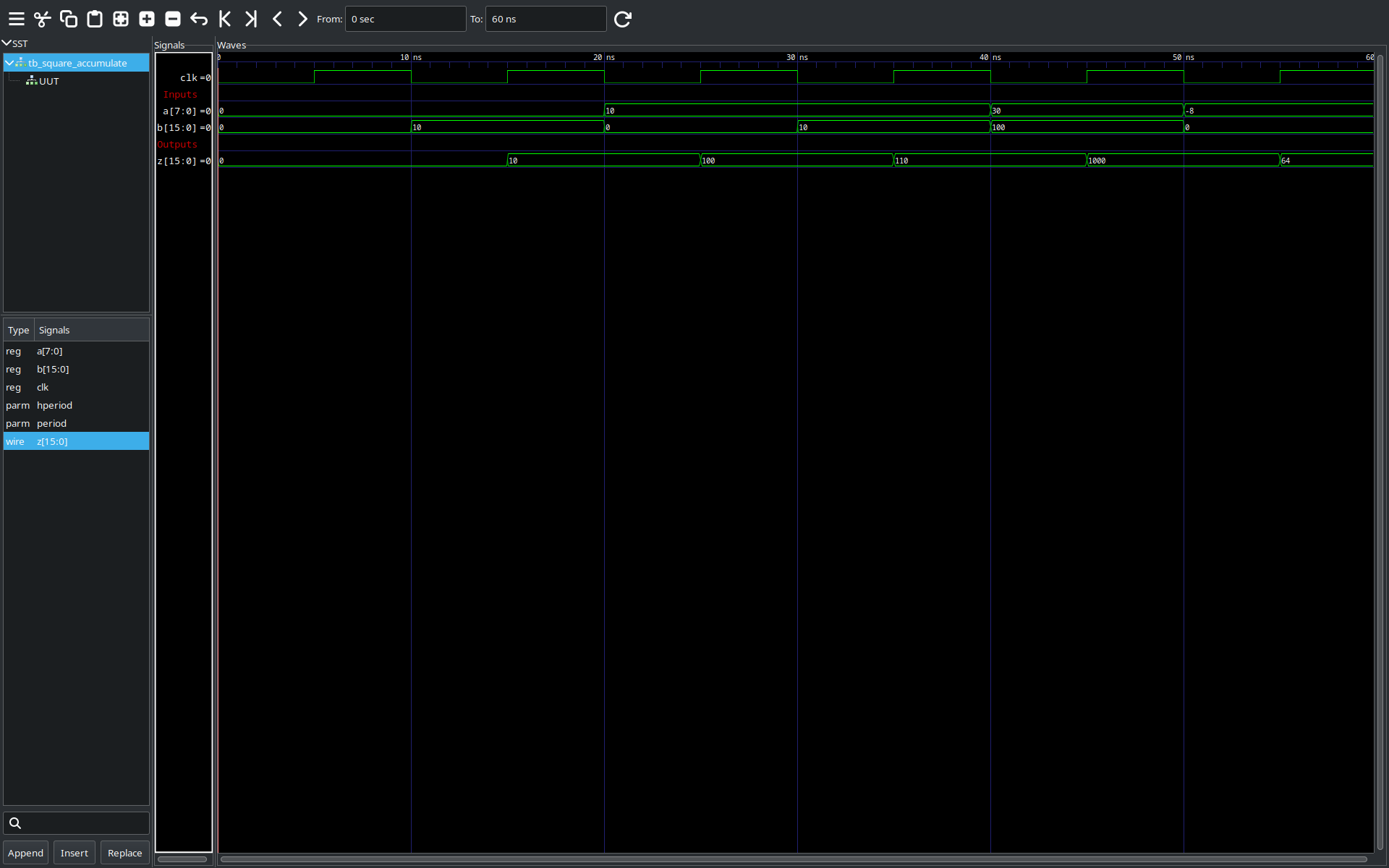
Compiling and running the testbench results in the expected output, and all the assertions are passed successfully.

1
2
3
4
5
6
7
8
9

$ iverilog -g2009 -o tb_square_accumulate tb_square_accumulate.sv ../rtl/square_accumulate.sv
$ ./tb_square_accumulate
VCD info: dumpfile tb_square_accumulate.vcd opened for output.
    0
   10
  100
  110
 1000
   64

GTKWave shows us the waveforms of our unit under test (click on the image to expand it).

Energy Calculation

The final testbench is for the calc_e module, which uses the calc_ck and square_accumulate modules internally. I have broken down the testbench into a four parts to make it easier to understand. The first part of the testbench looks very similar to the previous testbenches. First we instantiate the calc_e module (named UUT) with an input sequence width of 4 bits and output energy width of 16 bits. In this testbench we will be calculating the energy content of all 16 possible sequences of 4 bits, just like in the Python unit tests.

 1
 2
 3
 4
 5
 6
 7
 8
 9
10
11
12
13
14
15
16
17
18
19
20
21
22
23
24
25
26
27

module tb_calc_e;
    localparam period = 10;
    localparam hperiod = period/2;

    localparam SEQ_WIDTH = 4;
    localparam E_WIDTH = 16;

    reg clk;
    reg [SEQ_WIDTH-1:0] i_seq;
    reg  i_valid;
    wire [SEQ_WIDTH-1:0] o_seq;
    wire [E_WIDTH-1:0] o_e;
    wire o_valid;

    calc_e # (
        .SEQ_WIDTH(SEQ_WIDTH),
        .E_WIDTH(E_WIDTH)
    ) UUT (
        .clk(clk), 
        .i_seq(i_seq), 
        .i_valid(i_valid), 
        .o_seq(o_seq), 
        .o_e(o_e), 
        .o_valid(o_valid)
    );

    always #hperiod clk = ~clk;

The next part is to set up the array of expected output values. Using iverilog I was not able to initialize the array directly, so I had to assign it item by item instead.

 1
 2
 3
 4
 5
 6
 7
 8
 9
10
11
12
13
14
15
16
17
18
19

    integer expected[15:0];
    initial begin
        expected[0] = 14;
        expected[1] = 2;
        expected[2] = 2;
        expected[3] = 6;
        expected[4] = 2;
        expected[5] = 14;
        expected[6] = 6;
        expected[7] = 2;
        expected[8] = 2;
        expected[9] = 6;
        expected[10] = 14;
        expected[11] = 2;
        expected[12] = 6;
        expected[13] = 2;
        expected[14] = 2;
        expected[15] = 14;
    end

The next block generates the input sequences, with a new sequence being generated every cycle; at the start of the simulation we wait one clock cycle before generating the first input sequence. This block also controls the i_valid flag, which signals that the input to calc_e is valid.

 1
 2
 3
 4
 5
 6
 7
 8
 9
10
11
12
13
14

    initial begin
        clk = 0;
        i_seq = 0;
        i_valid = 0;

        #period; i_valid = 1;

        for (int i = 0; i < 16; i++) begin
            i_seq = i;
            #period;
        end

        i_valid = 0;
    end

The final block is similar to the previous testbenches; this block reads the output values from the calc_e module and compares them to the expected results. It also checks that the o_valid flag is set as expected and that the copy of the input sequence (o_seq) matches the actual input sequence. At the start of the block we must wait for one cycle to match the previous block, where only started generating valid input data after one clock cycle, and then we must wait for four clock cycles due to the latency of the calc_e module, which is equal to the width of the input sequence.

 1
 2
 3
 4
 5
 6
 7
 8
 9
10
11
12
13
14
15
16
17
18
19
20
21
22
23
24
25

    initial begin
        $dumpfile("tb_calc_e.vcd");
        $dumpvars(0,tb_calc_e);
        
        #period;
        #period;
        #period;
        #period;
        #period;
        
        assert(o_valid == 0);

        for (int i = 0; i < 16; i++) begin
            $display(o_e);
            assert(o_valid == 1);
            assert(o_seq == i);
            assert(o_e == expected[i]);
            #period;
        end

        assert(o_valid == 0);

        $finish();
    end
endmodule

We can compile the testbench (note that we have to pass in the sources files calc_ck.sv and square_accumulate.sv too) and run it in the terminal. Notice that this time we get a warning about a SystemVerilog feature which not yet supported by iverilog. Thankfully for us, the workaround it uses is fine for our purposes. From the output we can see that all the assertions pass, and the output from the $display commands matches our expected energy values.

 1
 2
 3
 4
 5
 6
 7
 8
 9
10
11
12
13
14
15
16
17
18
19
20
21
22
23
24
25
26
27

$ iverilog -g2009 -o tb_calc_e \
    tb_calc_e.sv \
    ../rtl/calc_ck.sv \
    ../rtl/calc_e.sv \
    ../rtl/square_accumulate.sv

../rtl/calc_e.sv:52: sorry: constant selects in always_* processes are not currently supported
(all bits will be included).

$ ./tb_calc_e
VCD info: dumpfile tb_calc_e.vcd opened for output.
   14
    2
    2
    6
    2
   14
    6
    2
    2
    6
   14
    2
    6
    2
    2
   14

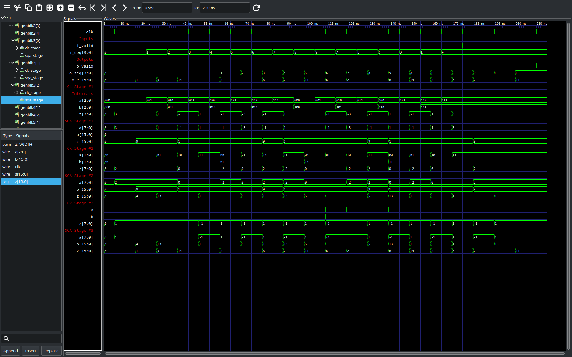
GTKWave shows us the waveforms of our testbench (click on the image to expand it). In this example I have included some internal signals from the calc_e module, specifically the inputs and outputs of the calc_ck and square_accumulates in all the internal stages.

Conclusion

In this post we have looked at design verification using a combination of high level models written in Python and hand-written testbenches written in SystemVerilog. The high level models can be used to better understand the problem at hand, and they can be used to verify the results from the RTL simulations. We have used Icarus Verilog to run our simulations and used the built-in $display and assert commands to verify the results of our units-under-test. We have also used GTKWave to visualise the waveforms which were dumped to a file by iverilog; these waveforms are very useful when debugging complex designs.

In the next post we will extend these concepts further by combining SystemVerilog and Python to write automated testbenches which can have increased test coverage.