Written by Wouter van Verre
on March 20, 2023

Searching for Low Autocorrelation Binary Sequences

In this post we will take a look at a numerical optimisation problem and how we might implement it on an FPGA. The problem in question is the search for binary sequences with low autorrelation values (Low-Autocorrelation Binary Sequences, or LABS for short). These sequences have applications in communications engineering, mathematics and statistical physics.

For more background reading, I would recommend one of the following papers:

The LABS Problem

In this blog I will not focus too much on the number theory, but I will provide a small summary to introduce the LABS problem. Consider a binary sequence $S$ of length $N$ such that $S = s_1s_2…s_{N}$ with $s_i \in \lbrace -1, 1\rbrace$. Then the autocorrelation values are defined as: $$ C_k(S) = \sum_{i=1}^{N-k}s_i s_{i+k} \tag{1} $$

For $k$ in range $0, 1, …, N - 1$; the sum of the squares of the off-peak ($k > 0$) correlation values is known as the energy of the sequence $S$: $$ E(S) = \sum_{k=1}^{N-1}C^2_k(S) \tag{2} $$

The LABS problem is defined as the search for the sequence $S$ of a given length $N$ with the minimum possible energy $E(S)$.

Searches based on heurististics, statistical analysis and even machine learning have been used to find long sequences with good energy values, but there is no guarantee that these methods will result in the lowest possible energy. To guarantee the optimal result for a given length it is necessary to evalulate all sequences of that length, which would require searching $2^N$ sequences. Based on number theory it is possible to show that sequences exist with three levels of symmetry, resulting in symmetry groups of upto 8 sequences, such that only one sequence in a symmetry group has to be evaluated. Some sequences in a group may be identical so not all groups are of size 8. Furthermore, the third level of symmetry is difficult to exploit in practical implementations. The first two levels of symmetry, however, are trivial to use, and as such it is possible to reduce the search space to size $2^{N-2}$.

The three types of symmetry are:

Inverting all the bits in the sequence
Inverting every other bit in the sequence (either all odd bit positons or all even bit positions)
Reversing the order of the sequence

The first two symmetries can be combined such that the value of the first two bits can be fixed. If we set the first two bits to $\lbrace -1, -1, \dots \rbrace$, all sequences with a different start can be mapped onto a sequence starting with $\lbrace -1, -1, \dots \rbrace$ using the first types of symmetry described above.

State of the arts implementations of search programs for the LABS problem use branch and bound techniques to reduce the search space further. In Mertens' 1996 paper the search space is reduced to size $O(1.85^N)$, for example. In this blog post we will focus purely on the FPGA implementation and how to optimize it. To keep things simple for the first post, we will consider the naive search implementation where we search the complete $2^{N-2}$ search space.

Example Calculation

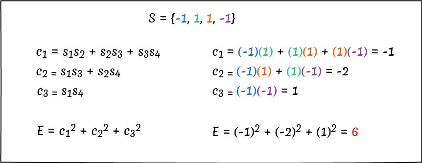
The image below contains an example of how to calculate the energy $E(S)$ for an example sequence of length 4. The sequence is $S = \lbrace -1, 1, 1, -1\ \rbrace$; the image shows the steps for calculating the correlation values $c_1, c_2, c_3$ and finally the energy content $E$.

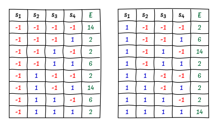
The next image shows a table with the results of an exhaustive search, showing the energy values of all sequences of length 4. The table shows the effect of the symmetry groups, as only three unique energy levels exist in the search space. Furthermore, it can be seen that every quarter of the table, with fixed values of $s_1$ and $s_2$, contains all three energy values at least once.

Figure 2. Energy content of all sequences of length 4.

Zeroes and Ones

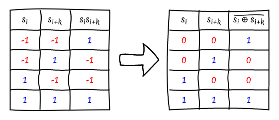
So far we have considered the LABS problem in its traditional, mathematical formulation, using the elements $\pm 1$. When implementing search applications in computers it is easier to consider the problem using the binary digits $\lbrace 0, 1 \rbrace$. We choose to map the element $-1$ to $0$, and $1$ to $1$; as shown in the table below, with this mapping the multiplication operation turns into the XNOR function.

Figure 3. Mapping the LABS problem onto binary digits.

Another potential approach for the calculation of $c_k$, instead of calculating the sum of all $s_i s_{i+k}$, is to count the number of pairs $(s_i, s_{i+k})$ where $s_i = s_{i_k}$ and by extension where $s_i \neq s_{i+k}$. Based on equation (1) above, he correlation value is the difference between these two counts since: $$ s_i s_{i+k} = \begin{cases} \phantom{-}1, s_i = s_{i+k}\\
-1, s_i \neq s_{i+k} \end{cases} \tag{4} $$ The sign of $c_k$ is not important, since we only care about the square of the value. We must take care to only consider the correct number of bits from the subcalculation $\overline{S \oplus (S > > k)}$. Considering equation (1) at the top of this page, we can see that for sequences of length $N$ the number of sequence elements (bits) under consideration is $L = N-k$. If $P$ is the count of pairs where $s_i$ is equal to $s_{i+k}$ then we must have $L - P$ pairs where the elements are not equal. The difference between these values is the correlation value: $$ C_k = 2P - L \tag {5} $$

The correlation value $c_k$ can also be calculated using logical right shifts ($> >$), XNOR and the population count function (POPCNT calculates the numbers of bits in a word set to 1) using the formula below: $$ c_k = 2 \times \texttt{POPCNT}(\overline{S \oplus (S > > k)}) - L \tag{3} $$ Here $(S > > k)$ has the effect of selecting bit $s_{i+k}$ and performing the XNOR operation with the bit $s_i$, which returns 1 for pairs where $s_i = s_{i+k}$. The POPCNT function then calculations the number of ones in the resulting binary word, which is the same as the number of equal pairs $P$ in Equation 5 above.

When implementing seach applications it is also typical to use zero-based indexing for the binary sequence, as opposed to one-based indexing in the original formulation. We thus define a binary sequence $S$ of length $N$ such that $S = s_0s_1…s_{N-1}$ with $s_i \in \lbrace 0, 1\rbrace$. Furthermore we generally write binary words with the most-significant bit on the left, and it feels intuitive to me to consider the most-significant bit to be $s_{N-1}$. Thus when considering a sequence as a binary word of $N$ bits, it would look as follows: $s_{N-1}s_{N-2}…{s_1}{s_0}$. This latter point is not actually very important, due to the third symmetry property mentioned earlier, we can reverse the order of the elements in the sequence and still expect the same energy value.

High Level Plan

I would like to design a fully pipelined FPGA module which takes a binary sequence as an input and calculates the energy content as defined above. We will then feed this module all $2^{N-2}$ sequences of interest, and continuously record the lowest energy value and the corresponding sequence. To interact with our LABS search module we will also add an AXI4-Lite interface.
The diagram below shows the high-level plan for our FPGA design.

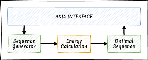
Figure 4. High-level overview of the LABS search application

The most interesting module in the diagram above is the energy calculation module. This is a fully pipelined module which accepts a new sample every clock cycle, and the latency through the module depends on the length of the sequence. As the input sequence progresses through the module a new correlation value is calculated every clock cycle, starting with $c_1$, $c_2$ and ending with $c_{N-1}$. In parallel with this we also update a running total of the energy content in the sequence using the correlation value calculated in the previous clock cycle. The diagram below shows how this ties together.

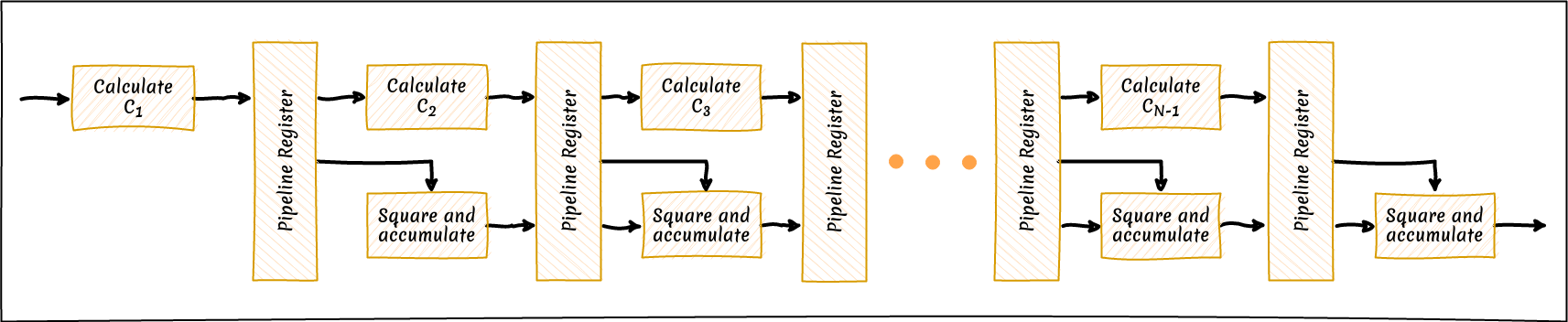
Figure 5. High-level overview of the energy calculation module

The running sum of the energy calculation is updated using the square accumulate blocks, which as the name suggests calculate the square of the $c_k$ value and add it into an accumulator register. The $c_k$ calculation block is a large LUT which maps the input sequence onto the $C_k$ values. In future posts we will consider how to optimise this part of the calculation further.

Implementation

This section will show the implementation (in SystemVerilog) of the components shown in Figure 5, which form the core of the LABS search application. In subsequent blog posts we will consider the supporting modules shown in Figure 4, and look at synthesis and implementation.

Correlation Calculation

The calc_ck module is shown in the code listing below. This module takes two sequences as an input: a and b. Here sequence a represents $S$ in equation (3), and sequence b represents $S » k$. The implementation takes one parameter, SEQ_WIDTH, which controls the width of these input sequences; the parent module will set this to the correct value, based on the length of the input sequence, $N$, and the value of $k$ for the specific instance. For the sake of simplicity I have chosen a fixed width of 8 bits for the output signal z. This is sufficient for input sequences of lengths upto 256 bits; in future we can come back to this to set the width dynamically based on the minimum width necessary at that stage.

In this case I have chosen to directly calculate the difference between pairs of equal and unequal elements, rather than using the XNOR-based approach described earlier. This module accepts values for a and b every clock cycle and delivers the result on the next clock cycle.

module calc_ck #
(
    parameter SEQ_WIDTH = 8
)
(
    input  wire                     clk,
    input  wire [SEQ_WIDTH-1:0]     a,
    input  wire [SEQ_WIDTH-1:0]     b,
    output reg  [7:0]               z
);

initial begin
    z = 0;
end

always_ff @(posedge clk) begin
    logic [7:0] temp;
    temp = 0;
    for (int i = 0; i < SEQ_WIDTH; i++) begin
        if (a[i] == b[i]) begin
            temp = temp + 1;
        end else begin
            temp = temp - 1;
        end
    end

    z <= temp;
end

endmodule

Square Accumulate

The next module under consideration is the square_accumulate module, which we discussed before. This module takes in two signals, a and b, and outputs one signal, z. Every clock cycle this module performs the following calculation: $z = s^2 + b$. We can chain two of these modules together by connecting the z output from the first module to the b input from the second module. By chaining together multiple instances of this module in this way, and connecting the output from calc_ck modules to their a inputs, we can implement the energy calculation shown in Equation (2).

The width of the input a is fixed at 8 bits, to match the width of the output from the calc_ck module; the width of the input b and output z can be controlled using the parameter Z_WIDTH. To ensure the square of the input value can be stored correctly, we extend the input signal to 16 bits after converting it to a signed decimal. It is signed because output from the current calc_ck implementation can be positive or negative. The implementation uses the * operator, leaving the FPGA toolchain to decide on the optimal implementation. This could be using DSP blocks or using LUTs; we will consider this further when we start running synthesis and implementation.

module square_accumulate #
(
    parameter Z_WIDTH = 16
)
(
    input  wire                 clk,
    input  wire [7:0]           a,
    input  wire [Z_WIDTH-1:0]   b,
    output reg  [Z_WIDTH-1:0]   z
);

initial begin
    z = 0;
end

wire signed [15:0] s;
assign s = 16'($signed(a));

always @(posedge clk) begin
    z <= $unsigned(s * s) + b;
end

endmodule

Energy Calculation

The final module to talk about in this blog post is the energy calculation module calc_e. This module calculates the energy content of input sequences (i_seq) of a given length (which is controlled by the parameter SEQ_WIDTH), and returns the energy content (o_e) alongside the original sequence (o_seq). The original sequence is returned so that we can store a copy of it if it has the lowest energy content so far. The module also has a pair of flags (i_valid/o_valid) to indicate whether the input and output values are valid.

The module contains three sets of pipeline registers: the original input signal is stored pl_ina, the shifted input signal in pl_inb, and the valid flag in pl_valid. The output values from the calc_ck and calc_e modules are already registered at the output, so we do not need additional pipeline registers in this module. The signals pl_ck and pl_e are thus wires, not registers.

Because the signals are registered at every stage, this module is able to accept one new sequence per clock cycle. The calc_e module contains $N - 1$ calc_ck and square_accumulate modules, one for every correlation value $c_k$ which has to be calculated. The total latency through the calc_e module is $N$ cycles, where $N$ is the number of bits in the input sequence.

The calc_e module is more complex than the previous modules, so I have decided to break it up into multiple parts to make it easier for me to explain what is going on.

module calc_e #
(
    parameter SEQ_WIDTH = 8,
    parameter E_WIDTH = 20
)
(
    input  wire                     clk,
    input  wire [SEQ_WIDTH-1:0]     i_seq,
    input  wire                     i_valid,
    output reg  [SEQ_WIDTH-1:0]     o_seq,
    output wire [E_WIDTH-1:0]       o_e,
    output wire                     o_valid
);

The first part of the code sets up the input and output ports for the module, no big suprises here.

    reg [SEQ_WIDTH-1:0] pl_ina [SEQ_WIDTH:0];
    reg [SEQ_WIDTH-1:0] pl_inb [(SEQ_WIDTH-1)-1:0];
    reg pl_valid [SEQ_WIDTH:0];

    wire [7:0] pl_ck [(SEQ_WIDTH-1)-1:0];
    wire [E_WIDTH-1:0] pl_e [SEQ_WIDTH-1:0];

assign o_e = pl_e[SEQ_WIDTH-1];
assign o_valid = pl_valid[SEQ_WIDTH];
assign o_seq = pl_ina[SEQ_WIDTH];

This block sets up the internal pipeline registers for the module: pl_ina for the original input sequence, pl_inb for the shifted input signal and pl_valid for the valid flag. There are also some pipeline wires to connect the outputs from the calc_ck and square_accumulate blocks. These are wires, not registers, since the signals are already registered in their respective modules. The final part of this piece of code assigns the last element in each pipeline to the output signals of the module.

genvar i;
generate for (i = 0; i < SEQ_WIDTH-1; i++) begin
    initial begin
        pl_inb[i] = 0;
    end
end endgenerate
generate for (i = 0; i <= SEQ_WIDTH; i++) begin
    initial begin
        pl_ina[i] = 0;
        pl_valid[i] = 0;
    end
end endgenerate

This block ensures that the pipeline registers are set to zero when the module is initialised.

generate for (i = 0; i < SEQ_WIDTH-1; i++) begin
    calc_ck # (.SEQ_WIDTH(SEQ_WIDTH-1-i)) ck_stage (.clk(clk), .a(pl_ina[i][SEQ_WIDTH-2-i:0]), .b(pl_inb[i][SEQ_WIDTH-2-i:0]), .z(pl_ck[i]));
    square_accumulate #(.Z_WIDTH(E_WIDTH)) sqa_stage (.clk(clk), .a(pl_ck[i]), .b(pl_e[i]), .z(pl_e[i+1]));
end endgenerate

This block creates $N-1$ stages (where $N$ is the width of the input sequences) of calc_ck and square_accumulate modules, and connects the inputs/outputs to the pipeline wires and registers.

assign pl_e[0] = 0;
always_comb begin
    pl_ina[0] = i_seq;
    pl_inb[0] = {1'b0, i_seq[SEQ_WIDTH-1:1]};
    pl_valid[0] = i_valid;
end

In this block we assign the first registers in each pipeline based on the input signals from the calc_e module. The first register in the energy pipeline is always set to zero, which sets the initial value of the accumulator.

generate for (i = 1; i < SEQ_WIDTH-1; i++) begin
    always @(posedge clk) begin
        pl_inb[i] <= {1'b0, pl_inb[i-1][SEQ_WIDTH-1:1]};
    end
end endgenerate

generate for (i = 1; i <= SEQ_WIDTH; i++) begin
    always @(posedge clk) begin
        pl_ina[i] <= pl_ina[i-1];
    end
end endgenerate

generate for (i = 1; i <= SEQ_WIDTH; i++) begin
    always @(posedge clk) begin
        pl_valid[i] <= pl_valid[i-1];
    end
end endgenerate

endmodule

In this final block we update the remaining elements in the pipeline registers. In the case of pl_valid and pl_ina we simply move the values one place further through the pipeline. In the case of pl_inb we shift the sequence by one bit every time we move the value further down the pipeline.

Summary

In this blog post I have introduced the Low-Autocorrelation Binary Sequence (LABS) problem, and I have explained how it can be mapped efficiently onto computer hardware. I have also worked out a high level plan on how we might implement the solution on an FPGA, and we have started to look at the implementation details for the proposed solution. More specifically we have shown example implementations for the core calculation blocks: calc_ck, square_accumulate and calc_E.

In the next blog post we will develop test benches for these three modules, so we can get some example waveforms and so that we can verify their implementations. In subsequent blog posts we will look at the supporting FPGA modules detailed in the high level plan, test benches for thos modules, synthesis and implementation on real FPGAs, and we will run this on one of my FPGA boards.

← → Top